Mango Leaf Image Classifier
Unleashing the Power of Convolutional Neural Networks:
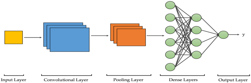
Convolutional Neural Networks (CNNs) are a specialized type of multi-layer neural networks designed specifically to analyze visual patterns directly from pixel images, requiring minimal preprocessing. CNNs have a unique architecture inspired by the visual cortex of living organisms, enabling them to achieve state-of-the-art results in various computer vision tasks. The building blocks of CNNs consist of two fundamental components: convolutional layers and pooling layers. Although these components are relatively simple, there are countless ways to arrange them to tackle specific computer vision problems effectively.
The key to understanding CNNs lies in comprehending their constituent elements, such as convolutional and pooling layers. Convolutional layers apply filters to input images, generating invariant features that are then passed on to subsequent layers. These features undergo further convolution with different filters in the next layer, creating increasingly invariant and abstract representations. This process continues until the final output, which represents features that are robust to occlusions and other variations.
The remarkable popularity of CNNs stems from their unique architecture, which eliminates the need for manual feature extraction. Instead, the network autonomously learns to extract relevant features from the data. This capability is achieved through the convolution operation, where images are convolved with filters to generate invariant features. This automated feature extraction, combined with the hierarchical nature of CNNs, enables them to effectively capture complex visual patterns.
In practice, the real challenge lies in designing optimal model architectures that make the best use of these simple yet powerful elements of convolutional neural networks. By carefully arranging convolutional and pooling layers, researchers and practitioners can achieve outstanding performance in various computer vision applications, such as object recognition, image classification, and image segmentation.
Algorithm Explanation
The given set of commands is used to download a dataset from Kaggle that contains information about mango leaf diseases. The commands install the Kaggle package, create a directory to store Kaggle API credentials, copy the necessary credentials to the appropriate directory, and download the dataset using the Kaggle API. Finally extracting the file content into 'images' folder.
                            !pip install kaggle
                            !mkdir -p ~/.kaggle
                            !cp kaggle.json ~/.kaggle/
                            !kaggle datasets download -d aryashah2k/mango-leaf-disease-dataset

                            #extracting files
                            from zipfile import ZipFile

                            with ZipFile('mango-leaf-disease-dataset.zip', 'r') as f:

                             #extract in different directory
                             f.extractall('images')
The code snippet organizes a set of images into train, validation, and test sets according to the specified ratios and moves them to their respective directories. It also removes any empty subfolders once the images have been moved.
    import os
    import shutil
    import random
    import tensorflow as tf
    import numpy as np
    import pandas as pd
    import matplotlib.pyplot as plt
    import seaborn as sns
    from pathlib import Path
    import glob
    import cv2

    root_directory = "/content/images"
    train_ratio = 0.7
    val_ratio = 0.15
    test_ratio = 0.15

    subfolders = [f.name for f in os.scandir(root_directory) if f.is_dir()]

    for subfolder in subfolders:
        subfolder_path = os.path.join(root_directory, subfolder)
        images = [f.name for f in os.scandir(subfolder_path) if f.is_file()]

        random.shuffle(images)

        num_images = len(images)
        num_train = int(num_images * train_ratio)
        num_val = int(num_images * val_ratio)
        num_test = num_images - num_train - num_val

        train_images = images[:num_train]
        val_images = images[num_train:num_train + num_val]
        test_images = images[num_train + num_val:]

        train_dir = os.path.join(root_directory, 'train', subfolder)
        val_dir = os.path.join(root_directory, 'val', subfolder)
        test_dir = os.path.join(root_directory, 'test', subfolder)
        os.makedirs(train_dir, exist_ok=True)
        os.makedirs(val_dir, exist_ok=True)
        os.makedirs(test_dir, exist_ok=True)

        for image in train_images:
            src = os.path.join(subfolder_path, image)
            dst = os.path.join(train_dir, image)
            shutil.move(src, dst)

        for image in val_images:
            src = os.path.join(subfolder_path, image)
            dst = os.path.join(val_dir, image)
            shutil.move(src, dst)

        for image in test_images:
            src = os.path.join(subfolder_path, image)
            dst = os.path.join(test_dir, image)
            shutil.move(src, dst)

        os.rmdir(subfolder_path) #deleting empty folders
  #optional code for debugging- can be excluded
  #testing whether the subfolders are formed after the above action
  data_dir_of_test = '../content/images/test'
  print(os.listdir(data_dir))

Creating the Pathlib PATH objects for train and validation and test dataset
      train_path = Path("/content/images/train")
      valid_path = Path("/content/images/val")
      test_path=Path("/content/images/test")
Finding the average size of images for considering resizing the images
        #finding the average size of images
from PIL import Image

data_folder = "/content/images/test"

total_width = 0
total_height = 0
num_images = 0

# Iterate over subfolders (labels)
for label in os.listdir(data_folder):
    label_folder = os.path.join(data_folder, label)
    if os.path.isdir(label_folder):
        # Iterate over image files in the label folder
        for image_file in os.listdir(label_folder):
            if image_file.endswith(".jpg") or image_file.endswith(".png"):
                # Open the image using PIL
                image_path = os.path.join(label_folder, image_file)
                image = Image.open(image_path)

                # Accumulate the width and height
                width, height = image.size
                total_width += width
                total_height += height
                num_images += 1

# Calculate the average width and height
avg_width = total_width / num_images
avg_height = total_height / num_images

# Print the average width and height
print("Average Width:", avg_width)
print("Average Height:", avg_height)
Average Width: 273.92333333333335 Average Height: 261.5283333333333
The given code snippet defines various variables related to a machine learning model for image processing. It includes parameters such as batch size, number of epochs, image channels, image dimensions, and paths to the training and validation dataset directories. These variables provide important information for training and evaluating the model on image data.
   batch_size = 72
epochs = 45
img_channel = 9
data_dir="../content/images"
img_width, img_height = (273.92,261.52)
train_dataset_main = data_dir + "/train"
valid_dataset_main = data_dir + "/val"
The create_dataset_df function is designed to create a pandas DataFrame from image files located in a specified main path directory. It iterates through the directories and subdirectories within the main path, collects the image paths and their corresponding class names, and returns a DataFrame with these details. This function helps organize image data into a tabular format for easier analysis and further processing.
    #creating DF's
    def create_dataset_df(main_path, dataset_name):
        print(f"{dataset_name} is creating ...")
        df = {"img_path":[],"class_names":[]}
        for class_names in os.listdir(main_path):
                for img_path in glob.glob(f"{main_path}/{class_names}/*"):
                    df["img_path"].append(img_path)
                    df["class_names"].append(class_names)
        df = pd.DataFrame(df)
        print(f"{dataset_name} is created !")
        return df
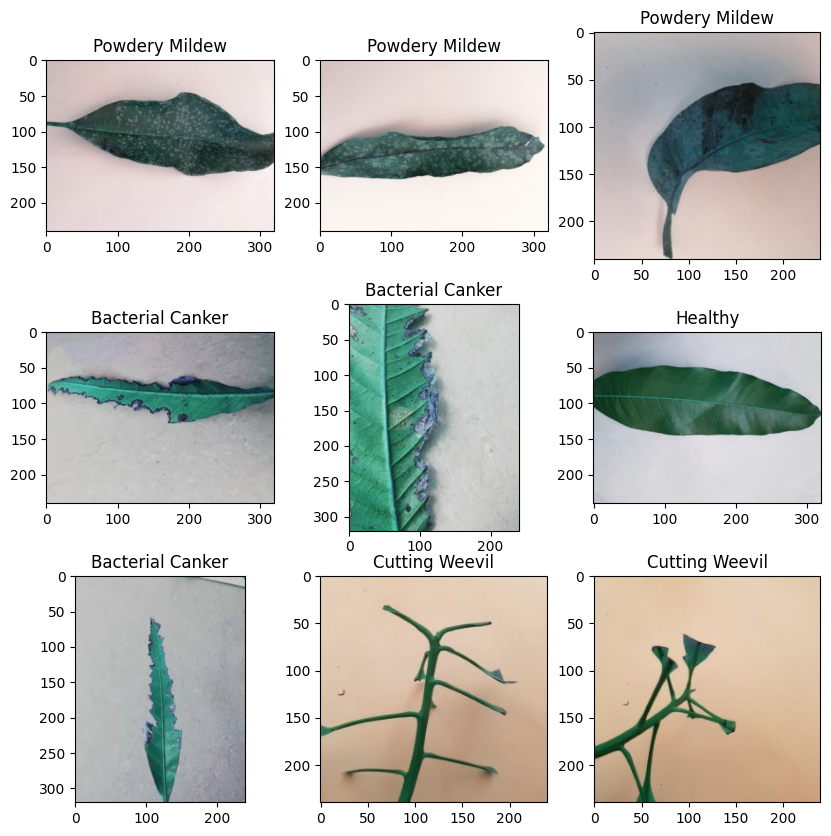
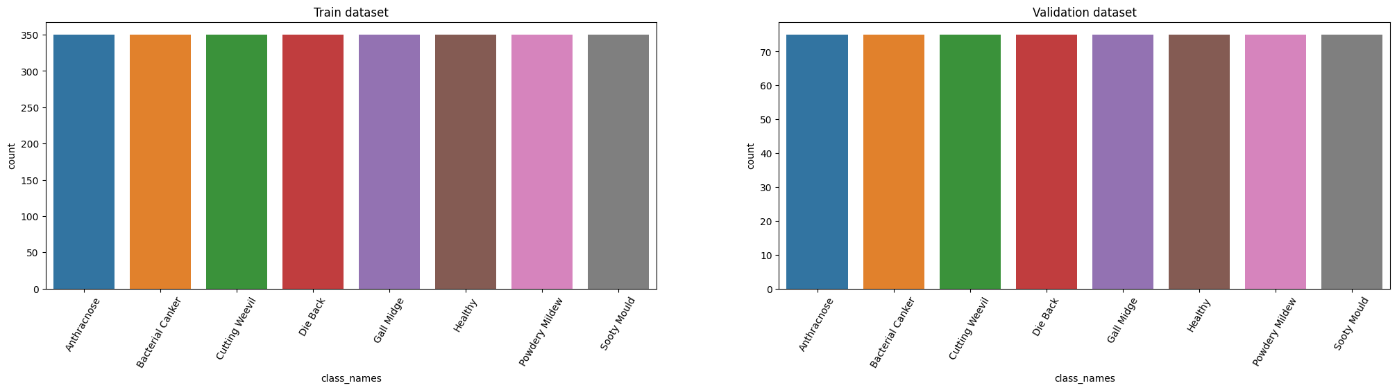
The code prepares the training and validation datasets by creating DataFrames, visualizes random images from the training dataset, displays the class distribution, encodes the class labels, applies one-hot encoding, calculates class weights, and retrieves the shape of an input image.
      train_df = create_dataset_df(train_dataset_main, "Train dataset")

      valid_df=create_dataset_df(valid_dataset_main, "Validation dataset")

      print(f"train samples: {len(train_df)} \n validation samples: {len(valid_df)}")
      def vizualizing_images(df,n_rows,n_cols):
          plt.figure(figsize=(10,10))
          for i in range(n_rows*n_cols):
              index = np.random.randint(0, len(df))
              img = cv2.imread(df.img_path[index])
              class_nm = df.class_names[index]
              plt.subplot(n_rows, n_cols, i+1)
              plt.imshow(img)
              plt.title(class_nm)
          plt.show()
      vizualizing_images(train_df, 3, 3)

      plt.figure(figsize=(25,5))
      # train dataset
      plt.subplot(1,2,1)
      sns.countplot(data=train_df.sort_values("class_names"),x="class_names")
      plt.title("Train dataset")
      plt.xticks(rotation = 60)
      # validation dataset
      plt.subplot(1,2,2)
      sns.countplot(data=valid_df.sort_values("class_names"),x="class_names")
      plt.title("Validation dataset")
      plt.xticks(rotation = 60)

      plt.show()

      from sklearn.preprocessing import LabelEncoder

      Le = LabelEncoder()
      train_df["class_names"] = Le.fit_transform(train_df["class_names"])

      #train_df["class_names"].value_counts()


      valid_df["class_names"] = Le.transform(valid_df["class_names"])
      #One Hot encoding
      train_labels = tf.keras.utils.to_categorical(train_df["class_names"])
      valid_labels = tf.keras.utils.to_categorical(valid_df["class_names"])
      train_labels[:10]
      train_labels.sum(axis=0)

      # Compute class weights

      classTotals = train_labels.sum(axis=0)
      classWeight = classTotals.max() / classTotals

      class_weight = {e : weight for e , weight in enumerate(classWeight)}
      print(class_weight)
      input_image = cv2.imread(train_df.img_path[0])

      input_image.shape
Train dataset is creating ... Train dataset is created ! Validation dataset is creating ... Validation dataset is created ! train samples: 2800 validation samples: 600
This code sets up the data loading and preprocessing pipelines, creates the training and validation datasets, builds a custom model architecture based on EfficientNetB2, and compiles the model for training.
def load(image , label):
image = tf.io.read_file(image)
image = tf.io.decode_jpeg(image , channels = 3)
return image , label
IMG_SIZE = 96
BATCH_SIZE = 64
# Basic Transformation
resize = tf.keras.Sequential([
tf.keras.layers.experimental.preprocessing.Resizing(IMG_SIZE, IMG_SIZE)
])
# Data Augmentation
data_augmentation = tf.keras.Sequential([
tf.keras.layers.experimental.preprocessing.RandomFlip("horizontal"),
tf.keras.layers.experimental.preprocessing.RandomRotation(0.1),
tf.keras.layers.experimental.preprocessing.RandomZoom(height_factor = (-0.1, -0.05))
])
# Function used to Create a Tensorflow Data Object
AUTOTUNE = tf.data.experimental.AUTOTUNE #to find a good allocation of its CPU budget across all parameters
def get_dataset(paths , labels , train = True):
image_paths = tf.convert_to_tensor(paths)
labels = tf.convert_to_tensor(labels)
image_dataset = tf.data.Dataset.from_tensor_slices(image_paths)
label_dataset = tf.data.Dataset.from_tensor_slices(labels)
dataset = tf.data.Dataset.zip((image_dataset , label_dataset))
dataset = dataset.map(lambda image , label : load(image , label))
dataset = dataset.map(lambda image, label: (resize(image), label) , num_parallel_calls=AUTOTUNE)
dataset = dataset.shuffle(1000)
dataset = dataset.batch(BATCH_SIZE)
if train:
dataset = dataset.map(lambda image, label: (data_augmentation(image), label) , num_parallel_calls=AUTOTUNE)
dataset = dataset.repeat()
return dataset
# Creating Train Dataset object and Verifying it
%time
train_dataset = get_dataset(train_df["img_path"], train_labels)
#iter() returns an iterator of the given object
#next() returns the next number in an iterator
image , label = next(iter(train_dataset))
print(image.shape)
print(label.shape)
# View a sample Training Image
print(Le.inverse_transform(np.argmax(label , axis = 1))[0])
plt.imshow((image[0].numpy()/255).reshape(96 , 96 , 3))
%time
val_dataset = get_dataset(valid_df["img_path"] , valid_labels , train = False)
image , label = next(iter(val_dataset))
print(image.shape)
print(label.shape)
# View a sample Validation Image
print(Le.inverse_transform(np.argmax(label , axis = 1))[0])
plt.imshow((image[0].numpy()/255).reshape(96 , 96 , 3))
# Building EfficientNet model
from tensorflow.keras.applications import EfficientNetB2
from tensorflow.keras.layers import Conv2D, BatchNormalization, Activation, MaxPooling2D, Dropout, Dense, Input, GlobalAveragePooling2D
backbone = EfficientNetB2(
input_shape=(96, 96, 3),
include_top=False
)
n = 64
model = tf.keras.Sequential([
backbone,
tf.keras.layers.Conv2D(128, 3, padding='same'),
tf.keras.layers.BatchNormalization(),
tf.keras.layers.Activation('relu'),
tf.keras.layers.Conv2D(64, 3, padding='same'),
tf.keras.layers.BatchNormalization(),
tf.keras.layers.Activation('relu'),
tf.keras.layers.Conv2D(32, 3, padding='same'),
tf.keras.layers.BatchNormalization(),
tf.keras.layers.Activation('relu'),
tf.keras.layers.GlobalAveragePooling2D(),
tf.keras.layers.Dense(128),
tf.keras.layers.Activation('relu'),
tf.keras.layers.Dropout(0.3),
tf.keras.layers.Dense(8, activation='softmax')
])
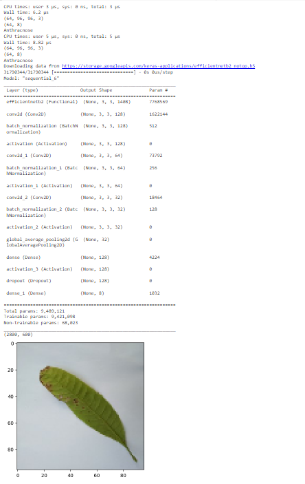
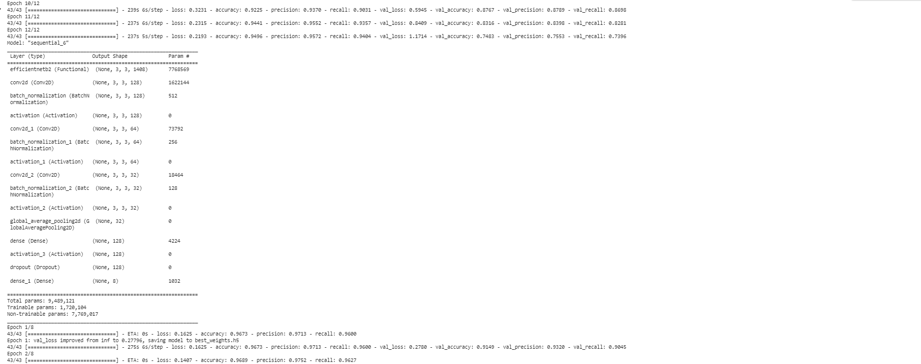
model.summary()
# Compiling your model by providing the Optimizer , Loss and Metrics
model.compile(
optimizer=tf.keras.optimizers.Adam(learning_rate=0.001, beta_1=0.9, beta_2=0.999, epsilon=1e-07),
loss = 'categorical_crossentropy',
metrics=['accuracy' , tf.keras.metrics.Precision(name='precision'),tf.keras.metrics.Recall(name='recall')]
)
#
len(train_labels),len(valid_labels)
The provided code trains a deep learning model using TensorFlow's Keras API. It incorporates an early stopping mechanism to monitor the accuracy during training and stops the training process if there is no improvement after a certain number of epochs. Additionally, it saves the best weights of the model based on the validation loss using a checkpoint callback. The first layer's weights are frozen to prevent further updates. The model is then trained for a specified number of epochs again, utilizing the checkpoint and early stopping callbacks. This approach ensures that the model is trained efficiently and stops early if there is no significant improvement in accuracy.
        early_stopping=tf.keras.callbacks.EarlyStopping(monitor="accuracy",patience=2,mode="auto")
        # Train the model
        history = model.fit(
            train_dataset,
            steps_per_epoch=len(train_labels)//BATCH_SIZE,
            epochs=12,
            callbacks=[early_stopping],
            validation_data=val_dataset,
            validation_steps = len(valid_labels)//BATCH_SIZE,
            class_weight=class_weight
        )
        model.layers[0].trainable = False
        # Defining our callbacks
        checkpoint = tf.keras.callbacks.ModelCheckpoint("best_weights.h5",verbose=1,save_best_only=True,save_weights_only = True)
        early_stop = tf.keras.callbacks.EarlyStopping(monitor="accuracy",patience=2)
        model.summary()


        # 2nd Train the model
        history = model.fit(
            train_dataset,
            steps_per_epoch=len(train_labels)//BATCH_SIZE,
            epochs=8,
            callbacks=[checkpoint , early_stop],
            validation_data=val_dataset,
            validation_steps = len(valid_labels)//BATCH_SIZE,
            class_weight=class_weight
        )
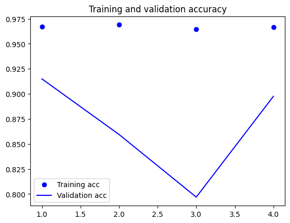
In order to assess the performance of a machine learning model, it is essential to visually examine the training and validation accuracy as well as the loss. In the provided code, this is accomplished by accessing the recorded accuracy and loss values stored in the 'history' object. Matplotlib, a popular data visualization library, is then employed to generate two plots: one illustrating the training and validation accuracy, and another depicting the training and validation loss. The appearance of the line plots is customized using the 'bo' and 'b' arguments to specify color and style. To enhance the interpretability of the plots, a legend is incorporated using the 'label' argument, providing clear labels for each line. Captions are added to the plots through the 'plt.title' function, and a legend is included utilizing the 'plt.legend' function. Finally, the 'plt.show' function is invoked to present the resulting plots.
            acc = history.history['accuracy']
            val_acc = history.history['val_accuracy']
            loss = history.history['loss']
            val_loss = history.history['val_loss']

            import matplotlib.pyplot as plt

            epochs = range(1, len(acc) + 1)

            plt.plot(epochs, acc, 'bo', label='Training acc')
            plt.plot(epochs, val_acc, 'b', label='Validation acc')
            plt.title('Training and validation accuracy')
            plt.legend()

            plt.figure()

            plt.plot(epochs, loss, 'bo', label='Training loss')
            plt.plot(epochs, val_loss, 'b', label='Validation loss')
            plt.title('Training and validation loss')
            plt.legend()

            plt.show()

            # history.history

My contribution to the code includes adding batch normalization and activation functions (BatchNormalization and Activation('relu')) after each Conv2D layer. These additions improve the stability and performance of the model by normalizing the layer inputs and introducing non-linearity. Batch normalization helps in reducing internal covariate shift and improves the generalization of the model. Activation functions introduce non-linearity, allowing the model to learn complex relationships between features. These enhancements contribute to the overall effectiveness and accuracy of the model in image classification tasks.
Implemented a sequential model using TensorFlow Keras, which is a high-level API for building and training deep learning models. The model has several layers that are used to extract and classify image features. It includes a pre-trained backbone, convolutional, activation, pooling, dense, dropout, and output layers. The pre-trained backbone helps the model learn important image features, and the convolutional layer applies 128 filters to the input image.
I have calculated average width and height of images to provide valuable insights into the characteristics of the dataset and assist in making informed decisions related to preprocessing, model design, and resource allocation, leading to better model performance and efficient training.
In order to enhance the performance of the machine learning model, I conducted experiments with different epoch sizes and carefully selected the most effective one. Determining the optimal epoch size involves considering factors such as model complexity, dataset size, and data noise. Through a systematic approach, I explored various epoch sizes to find the optimal point that achieves a balance between overfitting and underfitting. I iteratively trained the model with different epoch sizes and assessed its performance after each training cycle. This rigorous evaluation process enabled me to identify the ideal epoch size that maximizes the model's capabilities.
Note:I have implemented the image classifier using different approches and saved seperate notebooks as version 1 and version 2 in my github
Building an image classifier presented challenges in resizing images to balance detail preservation and avoid overfitting. Maintaining the aspect ratio was crucial to prevent distortion and artifacts. Selecting an appropriate image size involved finding the right balance to avoid loss of critical information or introducing noise. Data augmentation techniques were implemented to address overfitting and enhance generalization by introducing variability. Overcoming these challenges ensured an effective image classifier with accurate representations and improved performance on unseen images. My contribution to the code includes adding batch normalization and activation functions (BatchNormalization and Activation('relu')) after each Conv2D layer. These additions improve the stability and performance of the model by normalizing the layer inputs and introducing non-linearity. Batch normalization helps in reducing internal covariate shift and improves the generalization of the model. Activation functions introduce non-linearity, allowing the model to learn complex relationships between features. These enhancements contribute to the overall effectiveness and accuracy of the model in image classification tasks.
References
[1] https://levity.ai/blog/what-is-an-image-classifier
[2] https://www.kaggle.com/code/anand1994sp/facial-expression
[3] https://medium.com/analytics-vidhya/image-classification-techniques-83fd87011cac
[4] https://developer.apple.com/documentation/createml/creating-an-image-classifier-model
[5] https://www.geeksforgeeks.org/how-to-find-width-and-height-of-an-image-using-python/
[6] https://www.studytonight.com/python-howtos/how-to-unzip-file-in-python#:~:text=To%20unzip%20it%20first%20create,it%20will%20overwrite%20the%20path.
[7] https://www.tensorflow.org/tutorials/images/classification