Image Classifier
Overview
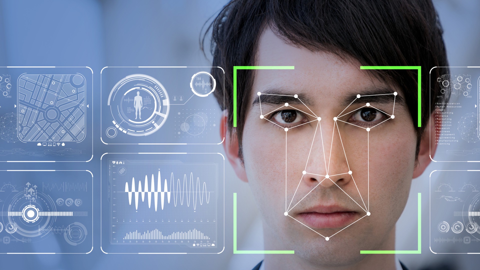
An image classifier is a type of machine learning model that is capable of identifying images. When provided with an image, it produces a category label for that image. To train an image classifier, you must present it with numerous examples of images that you have previously labeled. In this instance, we are teaching an image classifier to identify facial expressions by collecting pictures of various emotions like happiness, sadness, anger, disgust, fear, neutrality, and surprise.
Programming Process & Contribution
First, the code installs the kaggle package using pip. Then, it creates a directory called ~/.kaggle and copies a file named kaggle.json to this directory. The kaggle.json file contains authentication credentials that are required to download datasets from Kaggle. Next, the code uses the kaggle CLI to download a dataset called facial-emotion-expressions from Kaggle. The dataset is downloaded as a compressed ZIP file. Finally, the code uses the unzip command to extract the contents of the ZIP file, which can be used to train and evaluate an image classifier that can classify facial expressions based on the images in the dataset.
                            !pip install kaggle
                            !mkdir -p ~/.kaggle
                            !cp kaggle.json ~/.kaggle/
                            !kaggle datasets download -d samaneheslamifar/facial-emotion-expressions
                            !unzip facial-emotion-expressions.zip
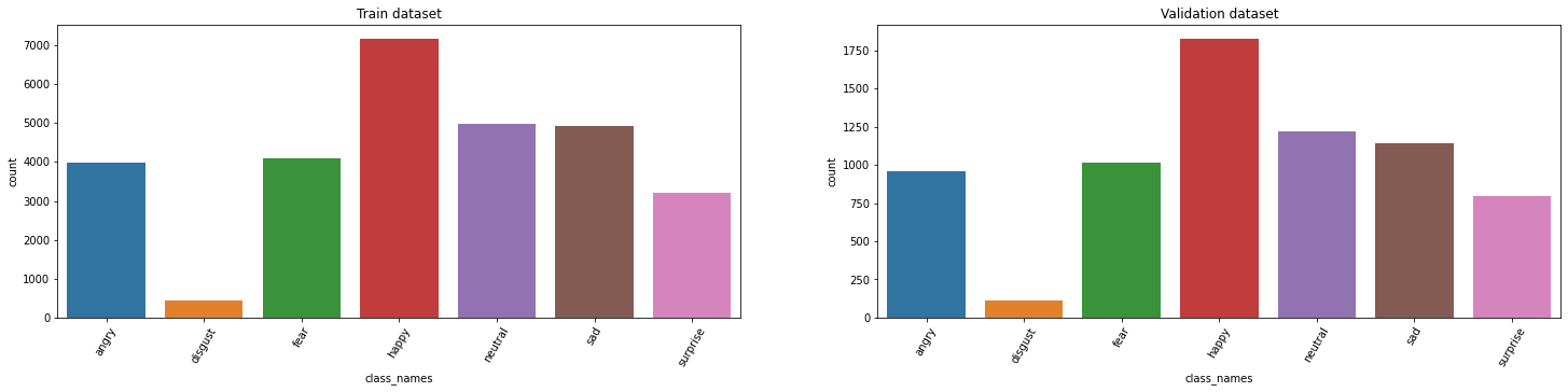
The code first sets the path for the dataset directory and prints the list of directories present in it. It then creates two lists for the names of classes in the training and validation datasets respectively. The next section sets the batch size, number of epochs, image channel, and dimensions for the input images. The code defines a function to create a dataset dataframe by iterating through the directories in the dataset path and populating the dataframe with the corresponding image path and class name. Two dataframes are created for the training and validation datasets using this function. The next part of the code displays a random sample of images from the training dataset using the vizualizing_images() function, which selects random images and their corresponding class names and displays them in a grid. Finally, a plot is created to visualize the distribution of classes in the training dataset.
    #[2] reference
    data_dir = '../input/facial-emotion-expressions/images'
    print(os.listdir(data_dir))
    classes_train = os.listdir(data_dir + "/train")
    classes_valid = os.listdir(data_dir + "/validation")
    print(f'Train Classes - {classes_train}')
    print(f'Validation Classes - {classes_valid}')

    # Creating the Pathlib PATH objects
    train_path = Path("/kaggle/input/facial-emotion-expressions/images/train")
    valid_path = Path("/kaggle/input/facial-emotion-expressions/images/validation")

    batch_size = 64
    epochs = 40
    img_channel = 3
    img_width, img_height = (48,48)
    train_dataset_main = data_dir + "/train"
    valid_dataset_main = data_dir + "/validation"
    def create_dataset_df(main_path, dataset_name):
        print(f"{dataset_name} is creating ...")
        df = {"img_path":[],"class_names":[]}
        for class_names in os.listdir(main_path):
                for img_path in glob.glob(f"{main_path}/{class_names}/*"):
                    df["img_path"].append(img_path)
                    df["class_names"].append(class_names)
        df = pd.DataFrame(df)
        print(f"{dataset_name} is created !")
        return df
    train_df = create_dataset_df(train_dataset_main, "Train dataset")

    valid_df=create_dataset_df(valid_dataset_main, "Validation dataset")
    train_df.sample(5)
    valid_df.sample(5)
    print(f"train samples: {len(train_df)} \n validation samples: {len(valid_df)}")
    def vizualizing_images(df,n_rows,n_cols):
        plt.figure(figsize=(10,10))
        for i in range(n_rows*n_cols):
            index = np.random.randint(0, len(df))
            img = cv2.imread(df.img_path[index])
            class_nm = df.class_names[index]
            plt.subplot(n_rows, n_cols, i+1)
            plt.imshow(img)
            plt.title(class_nm)
        plt.show()
    vizualizing_images(train_df, 3, 3)

    plt.figure(figsize=(20,6))
The code is used to check if there are any GPUs available and if so, it sets the first available GPU as the default device for TensorFlow operations. First, the code creates a list of all available physical devices and assigns it to the variable gpus. Then, it checks if the length of the gpus list is greater than zero, which indicates that at least one GPU is available. If a GPU is available, the code sets the first GPU as the default device for TensorFlow operations using the tf.device() function. This ensures that TensorFlow will use the GPU for computations instead of the CPU, which can significantly speed up training and inference of deep learning models.
        gpus = tf.config.list_physical_devices('GPU')
        if len(gpus) > 0:
          tf.device(gpus[0])
The code snippet implements an image classification model based on the EfficientNetB2 architecture. It begins by defining a function to decode and load image files, and then sets constants for image size and batch size. The code then applies a basic transformation to resize images and a data augmentation pipeline that includes horizontal flip, random rotation, and random zoom. It also creates a TensorFlow data object from the image paths and labels, applies the transformation pipeline, shuffles, batches, and augments the data (if required). The model consists of EfficientNetB2 as the backbone, followed by a convolutional layer, global average pooling, and two fully connected layers. Finally, the model is compiled with an optimizer, loss function, and metrics.
        # Function used for Transformation [2]

        def load(image , label):
            image = tf.io.read_file(image)
            image = tf.io.decode_jpeg(image , channels = 3)
            return image , label

        # Define IMAGE SIZE and BATCH SIZE
        IMG_SIZE = 96
        BATCH_SIZE = 64

        # Basic Transformation
        resize = tf.keras.Sequential([
            tf.keras.layers.experimental.preprocessing.Resizing(IMG_SIZE, IMG_SIZE)
        ])

        # Data Augmentation
        data_augmentation = tf.keras.Sequential([
            tf.keras.layers.experimental.preprocessing.RandomFlip("horizontal"),
            tf.keras.layers.experimental.preprocessing.RandomRotation(0.1),
            tf.keras.layers.experimental.preprocessing.RandomZoom(height_factor = (-0.1, -0.05))
        ])

        # Function used to Create a Tensorflow Data Object
        AUTOTUNE = tf.data.experimental.AUTOTUNE #to find a good allocation of its CPU budget across all parameters
        def get_dataset(paths , labels , train = True):
            image_paths = tf.convert_to_tensor(paths)
            labels = tf.convert_to_tensor(labels)

            image_dataset = tf.data.Dataset.from_tensor_slices(image_paths)
            label_dataset = tf.data.Dataset.from_tensor_slices(labels)

            dataset = tf.data.Dataset.zip((image_dataset , label_dataset))

            dataset = dataset.map(lambda image , label : load(image , label))
            dataset = dataset.map(lambda image, label: (resize(image), label) , num_parallel_calls=AUTOTUNE)
            dataset = dataset.shuffle(1000)
            dataset = dataset.batch(BATCH_SIZE)

            if train:
                dataset = dataset.map(lambda image, label: (data_augmentation(image), label) , num_parallel_calls=AUTOTUNE)
                dataset = dataset.repeat()

            return dataset

        # Creating Train Dataset object and Verifying it
        %time
        train_dataset = get_dataset(train_df["img_path"], train_labels)

        #iter() returns an iterator of the given object
        #next() returns the next number in an iterator
        image , label = next(iter(train_dataset))
        print(image.shape)
        print(label.shape)
        # View a sample Training Image
        print(Le.inverse_transform(np.argmax(label , axis = 1))[0])
        plt.imshow((image[0].numpy()/255).reshape(96 , 96 , 3))


        %time
        val_dataset = get_dataset(valid_df["img_path"] , valid_labels , train = False)

        image , label = next(iter(val_dataset))
        print(image.shape)
        print(label.shape)

        # View a sample Validation Image
        print(Le.inverse_transform(np.argmax(label , axis = 1))[0])
        plt.imshow((image[0].numpy()/255).reshape(96 , 96 , 3))


        # Building EfficientNet model
        from tensorflow.keras.applications import EfficientNetB2
        from tensorflow.keras.layers import Conv2D, BatchNormalization, Activation, MaxPooling2D, Dropout, Dense, Input, GlobalAveragePooling2D


        backbone = EfficientNetB2(
            input_shape=(96, 96, 3),
            include_top=False
        )

        n = 64
        model = tf.keras.Sequential([
            backbone,
            tf.keras.layers.Conv2D(128, 3, padding='same'),
            tf.keras.layers.LeakyReLU(alpha=0.2),
            tf.keras.layers.GlobalAveragePooling2D(),
            tf.keras.layers.Dense(128),
            tf.keras.layers.LeakyReLU(alpha=0.2),
            tf.keras.layers.Dropout(0.3),
            tf.keras.layers.Dense(7, activation='softmax')
        ])

        model.summary()

        # Compiling your model by providing the Optimizer , Loss and Metrics
        model.compile(
            optimizer=tf.keras.optimizers.Adam(learning_rate=0.001, beta_1=0.9, beta_2=0.999, epsilon=1e-07),
            loss = 'categorical_crossentropy',
            metrics=['accuracy' , tf.keras.metrics.Precision(name='precision'),tf.keras.metrics.Recall(name='recall')]
        )
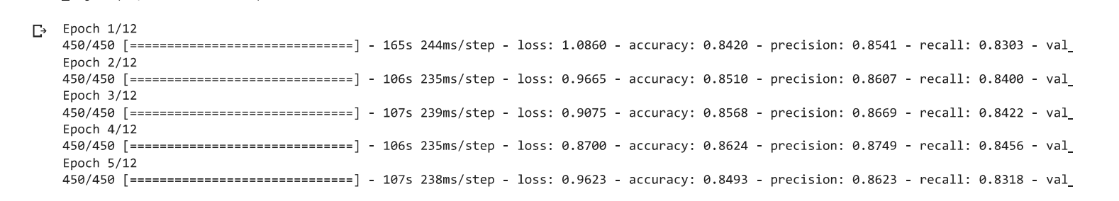
This code trains an image classification model based on the EfficientNetB2 architecture using the fit method in TensorFlow. It employs the early_stopping callback function, which halts the training process if the validation accuracy fails to improve over two consecutive epochs. Two training cycles are performed using different callbacks. The first one uses the early_stopping function for 12 epochs, and the ModelCheckpoint callback saves the best weights obtained. Subsequently, to avoid overfitting, the first layer of the model is frozen, and the best weights are used to retrain the model for 8 epochs, while early_stopping is active. Finally, the model is evaluated on the validation set, and its training and validation accuracy and loss metrics are saved in the history variable.
        #[2]
        early_stopping=tf.keras.callbacks.EarlyStopping(monitor="accuracy",patience=2,mode="auto")
        # Train the model
        history = model.fit(
            train_dataset,
            steps_per_epoch=len(train_labels)//BATCH_SIZE,
            epochs=12,
            callbacks=[early_stopping],
            validation_data=val_dataset,
            validation_steps = len(valid_labels)//BATCH_SIZE,
            class_weight=class_weight
        )
        model.layers[0].trainable = False
        # Defining our callbacks
        checkpoint = tf.keras.callbacks.ModelCheckpoint("best_weights.h5",verbose=1,save_best_only=True,save_weights_only = True)
        early_stop = tf.keras.callbacks.EarlyStopping(monitor="accuracy",patience=2)
        model.summary()


        # 2nd Train the model
        history = model.fit(
            train_dataset,
            steps_per_epoch=len(train_labels)//BATCH_SIZE,
            epochs=8,
            callbacks=[checkpoint , early_stop],
            validation_data=val_dataset,
            validation_steps = len(valid_labels)//BATCH_SIZE,
            class_weight=class_weight
        )
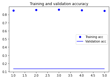
To evaluate the performance of a machine learning model, it is crucial to visualize its training and validation accuracy and loss. In order to achieve this, the recorded accuracy and loss values during model training can be accessed through the 'history' object in the provided code. The Matplotlib library is then utilized to create two plots; the first plot displays the training and validation accuracy, while the second plot displays the training and validation loss. The color and style of the line plots are defined by using the 'bo' and 'b' arguments, and a legend is added to the plot using the 'label' argument. To provide further context to the plots, a title is added using the 'plt.title' function, and a legend is included with the 'plt.legend' function. Lastly, the 'plt.show' function is called to display the resulting plots.
            acc = history.history['accuracy']
            val_acc = history.history['val_accuracy']
            loss = history.history['loss']
            val_loss = history.history['val_loss']

            import matplotlib.pyplot as plt

            epochs = range(1, len(acc) + 1)

            plt.plot(epochs, acc, 'bo', label='Training acc')
            plt.plot(epochs, val_acc, 'b', label='Validation acc')
            plt.title('Training and validation accuracy')
            plt.legend()

            plt.figure()

            plt.plot(epochs, loss, 'bo', label='Training loss')
            plt.plot(epochs, val_loss, 'b', label='Validation loss')
            plt.title('Training and validation loss')
            plt.legend()

            plt.show()

            # history.history

Google Colab provides two options for running code on a remote server: using a CPU or a GPU. A CPU is the primary processor in a computer, while a GPU is specialized for complex mathematical operations and is particularly useful for machine learning tasks involving large amounts of data. Although a GPU in Colab can significantly speed up the training process, it may come at a cost, as Colab provides a limited amount of free GPU usage, and additional usage may require payment. Conversely, using a CPU in Colab is entirely free and does not have usage limitations. Therefore, the choice between using a CPU or GPU in Google Colab depends on the size of the dataset and the complexity of the computations involved in the machine learning tasks. I have implemented the notebook using GPU as my runtime and observed the difference in the runtime thus increasing the efficiency.
Contributed in improving the accuracy by replacing ReLU with LeakyReLU. LeakyReLU is an activation function used in neural networks, and it differs from ReLU by introducing a small negative slope for negative inputs rather than setting them to zero. The small slope is designed to prevent the "dying ReLU" problem, which occurs when some neurons become inactive during training and cannot recover, leading to reduced effectiveness. LeakyReLU ensures that the gradient will never be zero, allowing the network to continue learning, even when some neurons output negative values. In summary, LeakyReLU is preferred over ReLU because it addresses the "dying ReLU" problem and has been shown to improve the performance of deep neural networks.
Implemented a sequential model using TensorFlow Keras, which is a high-level API for building and training deep learning models. The model has several layers that are used to extract and classify image features. It includes a pre-trained backbone, convolutional, activation, pooling, dense, dropout, and output layers. The pre-trained backbone helps the model learn important image features, and the convolutional layer applies 128 filters to the input image. The LeakyReLU activation function with an alpha value of 0.2 is applied to the output of the convolutional layer, followed by a global average pooling layer, a dense layer with 128 units, another LeakyReLU activation function, a dropout layer with a rate of 0.3, and an output layer with 7 units and a softmax activation function. Overall, this model is suitable for multi-class classification tasks involving image data.
Apart from above contribution, I have implemented different approaches but none have improved the accuracy that I have got from the leakyReLU. When implemented Batch Normalization I have seen drastic downfall of accuracy.
To optimize the performance of the machine learning model, I have experimented with different epoch sizes and selected the best one. The optimal epoch size depends on various factors such as model complexity, dataset size, and noise in the data. By trying different epoch sizes, I have identified the best spot that balances the trade-off between overfitting and underfitting. I have trained the model with a range of epoch sizes and evaluated the performance after each epoch.
References
[1] https://levity.ai/blog/what-is-an-image-classifier
[2] https://www.kaggle.com/code/anand1994sp/facial-expression